Where's my repo? Using the GitHub app

Sharing code with the internets is made possible with GitHub. In a previous post I outlined how to add, commit and push code on GitHub via Git Bash, a scary looking terminal that sane people avoid. I’ve since played with the GitHub app which makes sharing even easier. Here I will create a repo and share my Fitbit R data wrangling code.

I’ve assumed one has a GitHub account and the GitHub app installed. I first need to create a repo. On the GitHub site I clicked on the “+” symbol and selected “New repository”. There’s also a helpful green “New repository” button which would have saved me one click. 

I entered “fitbit” as my repository name then selected “Create repository” at the bottom.

On the next screen (above) I selected “Set up in Desktop”. An “External Protocol Request” popup appeared and I selected “Launch Application”. Then magic happened. Magic. I was prompted to select where I wished to place my repo on my local machine (below). My repos exist under Documents > GitHub. Hitting OK, the repo cloned. My fitbit repo appeared on the left hand side of the GitHub app. 

Browsing to the fitbit repo directory on my local, I pasted the code I wish to share.

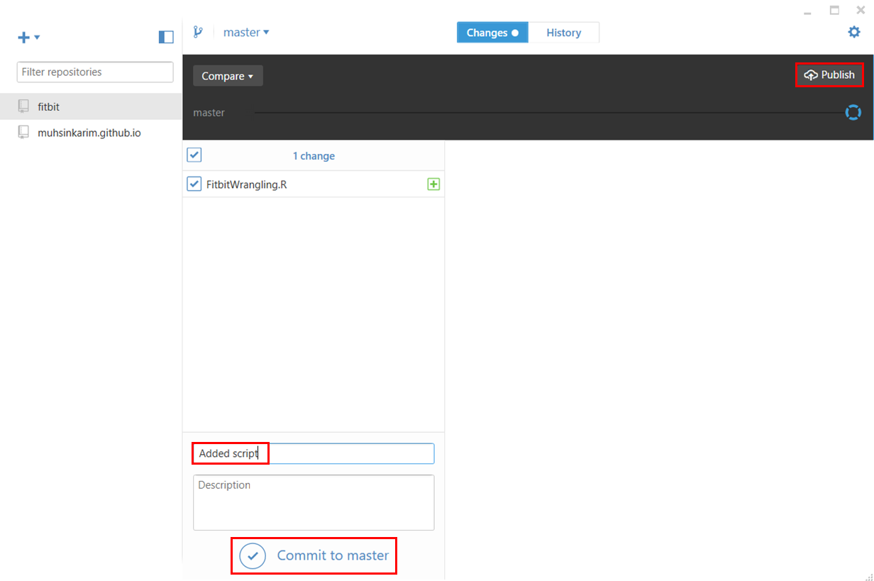
Returning to the GitHub app, it’s detected the addition of my script. I enter something in the “Summary” text field then select “Commit to master” below the “Publish” top right.

Then returning to GitHub, I hit refresh on my fitbit repo, and boom! My script appears on the internets. As I make changes to the script on my local, the GitHub app will allow me to commit changes and publish online.

Fitbit 02 – Getting and wrangling sleep data

Previous post in this series: Fitbit 01 – Getting and wrangling weight, steps and calories burned data.

Let’s continue to get and wrangle Fitbit data. This post will tackle sleep data and address my unattractive trait of not easily letting things go.

I applied the following R package fitbitScraper function wrapped in a data frame:

dfSleep <- as.data.frame(get_sleep_data(cookie, start_date = startDate, end_date = endDate))

There’s a lot of data. Below is the list of columns I want to keep:

• df.startDateTime – The start datetime of sleep.
• df.endDateTime – The end datetime of sleep.
• df.sleepDuration – The minutes between the start and end time. df.sleepDuration = df.awakeDuration + df.restlessDuration + df.minAsleep".
• df.awakeDuration – The minutes of wakefulness.
• df.restlessDuration – The minutes of restlessness.
• df.minAsleep – The minutes of actual sleep. I want to maximise this data field. More sleep less grumpiness.

If you’re a normalish human being, you would look at the sleep data and examine it for any anomalies. Your keen eye will note that some sleep durations are split across two or more sessions. That is, you went to bed, woke up in the middle of the night, then fell asleep again. Depending on how long you were awake for, Fitbit will record separate sessions.

I am working towards a tidy dataset with each row representing a unique date with the day’s Fitbit data. Separate sleep sessions cause duplicate dates. Being a normalish human being, you write code that will group the split sleep sessions back together. Unique dates per sleep lends to tidy data.

If you’re not a normal human being, you examine the intricate nature of these split sleep sessions and spend way too much time writing code that groups the data back together.

I am not a normal human being.

Split sessions occur for two reasons. The first occurs when I wake up in the early hours of the morning. An example is below.

On the night of the 22^nd March I fell asleep at 23:37. I woke up at 3:49 on the 23^rd. After hating my life and eating morning chocolate, I finally fell asleep again at 4:51. Technically the second session date should be displayed as the 23^rd of March, not the 22^nd. These display dates are akin to the “date I tried to fall asleep”. The datetimes record the true date and times.

When I combine these separate sessions, the new sleep start time will be 23:37 and the new sleep end time will be 07:46. The SleepDuration, SleepAwakeDuration, SleepRestlessDuration, SleepMinAsleep, SleepAwakeCount and SleepRestlessCount values will be summed together. I would also like to note the number of minutes I spent awake between sessions and the number of separate sessions (two in this example).

The second split sleep session type appears to be a glitch with sessions being separated by a difference of one minute. An example is below. 

On the 23^rd of February I have sleep sessions ending at 03:47 then resuming at 03:38. There are multiple instances where this occurs in my datasets. As before, the sleep variables from both sessions will be summed. I don’t need to note the minutes between the sessions as the one minute difference is meaningless. Further, the number of sleep sessions should be recorded as one, not two.

There’s a final consideration with split sleep sessions. Consider the below.

According this this display, on the 8th April I slept from 22:23 to 5:27, then on the 21:06 to the 23:57 on the same day. No I didn’t! The sleep session datetimes are overlapping. The session displayed on the 8th April from 21:06 to 23:57 should read the 9th April, not the 8th. This session needs to be combined with the sessions displayed on the 9th April from the 23:58 to 6:03. I may not be a normal human being, but I have my limits. For this last case, I did not write a patch of code that could group the data appropriately. Since there were few instances when such overlapping sessions occurred, I let it go – such sessions were removed from the dataset resulting in missing sleep data for that particular date.

Here is a quick plot of the average number of minutes asleep per weekday. Nothing out of the ordinary. I sleep an average 7.6 hours on Sunday nights and an average 6.4 hours on Wednesday nights. I can’t think of a reason why I get fewer hours on a Wednesday night. 

I spend most of my time wrangling data. I come across problems in datasets as described above often, and write code to return the numbers back to reality as much as possible. When the costs (time and effort) outweigh the benefits (more clean data) I have to let some data go and remove it.

I have outlined the code at the end of this post for the avid reader.

#### Sleep        
        
    ### Get data
    
        dfSleep <- as.data.frame(get_sleep_data(cookie, start_date = startDate, end_date = endDate))


    ### Keep key columns
    
        dfSleep <- dfSleep[ , c("df.date", "df.startDateTime", "df.endDateTime", "df.sleepDuration", "df.awakeDuration", 
                                "df.restlessDuration", "df.minAsleep")]

        ## Rename colnames
        # Date is sleep date attempt
        colnames(dfSleep) <- c("Date","SleepStartDatetime", "SleepEndDatetime", "SleepDuration", 
                               "SleepAwakeDuration", "SleepRestlessDuration", "SleepMinAsleep")


    ### Combine the split sleep sessions
    
        ## Index the Dates that are duplicated along with their original
        duplicatedDates <- unique(dfSleep$Date[which(duplicated(dfSleep$Date))])
        dfSleep$Combine <- ""
        dfSleep$Combine[which(dfSleep$Date %in% duplicatedDates)] <- 
            dfSleep$Date[which(dfSleep$Date %in% duplicatedDates)]
        
        ## Subset the combine indexed rows
        dfSubset <- dfSleep[which(dfSleep$Combine != ""), ]

        ## Aggregate rows marked to combine
        dfSubset <- 
            dfSubset %>%
            group_by(Combine) %>%
            summarise(Date = unique(Date),
                      SleepStartDatetime = min(SleepStartDatetime), # Earliest datetime
                      SleepEndDatetime = max(SleepEndDatetime), # Latest datetime
                      SleepDuration = sum(SleepDuration),
                      SleepAwakeDuration = sum(SleepAwakeDuration),
                      SleepRestlessDuration = sum(SleepRestlessDuration),
                      SleepMinAsleep = sum(SleepMinAsleep),
                      SleepSessions = n() # Number of split sleep sessions
            )


    ### Get the minutes awake between split sessions    
    
        ## Calculate sleep duration using start and end time using floor (round down)
        dfSubset$AwakeBetweenDuration <- floor((as.POSIXct(dfSubset$SleepEndDatetime) - as.POSIXct(dfSubset$SleepStartDatetime)) * 60)
        dfSubset$AwakeBetweenDuration <- dfSubset$AwakeBetweenDuration - dfSubset$SleepDuration
        
        ## Set any duration less than five minutes to zero
        dfSubset$AwakeBetweenDuration[which(dfSubset$AwakeBetweenDuration < 5)] <- 0


    ### Remove rows of combined sleep sessions
    
        ## Remove any row with AwakenBetweenDuration greater than five hours
        dfSubset <- dfSubset[-which(dfSubset$AwakeBetweenDuration > 60*5), ]


    ### Replace split sessions in dfSleep with dfSubset
    
        ## Prepare dfSubset for merging
        
        ## Remove duplicate dates from dfSleep
        dfSleep <- dfSleep[-which(nchar(dfSleep$Combine) > 0), ]
        
        ## Add new columns
        dfSleep$SleepSessions <- 1
        dfSleep$AwakeBetweenDuration <- 0
        
        ## Remove Combine column
        dfSubset <- dfSubset[ , -which(colnames(dfSubset) == "Combine")]
        dfSleep <- dfSleep[ , -which(colnames(dfSleep) == "Combine")]
        
        ## Bind dfSubset
        dfSleep <- rbind.data.frame(dfSleep, dfSubset)

        
    ### Coerce as date
        
        dfSleep$Date <- as.Date(dfSleep$Date)

Fitbit 01 – Getting and wrangling weight, steps and calories burned data

I love my Fitbit Charge HR [1]. It tracks my steps, it tracks my heartbeat. It tracks my sleep hours. Alas it does not keep me warm at night unless if malfunctions, bursts into flames then rudely singes my beard.

I’m keen to analyse my Fitbit data to gain some insight into my biology and behaviour. What days and times am I the most active? What drives my weight gain and loss? What do I need to do to get a decent night’s sleep? I will attempt to answer such questions through a series of Fitbit posts, each one taking a snapshot of the process from data to insights. This post is focussed on getting the Fitbit data, then wrangling it into tidy data for further visualisation and analysis.

Accessing my Fitbit data is made easy with the R package fitbitScraper. I have been using my Fitbit since March 2015. I have been recording my weight via the Fitbit Aria Wi-Fi Smart Scale since the end of September 2015. I will analyse data from October 2015 (a complete month since recording my weight) to March 2016 (seven months). These are the data variables of interest:

• Weight 
• Sleep 
• Steps 
• Distance 
• Activity 
• Calories burned 
• Heartbeat. 

I will focus on weight, steps and calories burned for this post.

Weight

After authenticating [2], assigning my start and end date, I applied the get_weight_data function and received the following output:

 

> get_weight_data(cookie, start_date = startDate, end_date = endDate)

                  time weight

1  2015-09-27 23:59:59   72.8

2  2015-10-04 23:59:59   73.6

3  2015-10-11 23:59:59   74.5

4  2015-10-18 23:59:59   74.5

5  2015-10-25 23:59:59   74.5

6  2015-11-01 23:59:59   74.0

7  2015-11-08 23:59:59   73.3

8  2015-11-15 23:59:59   73.4

9  2015-11-22 23:59:59   74.3

10 2015-11-29 23:59:59   73.1

11 2015-12-06 23:59:59   72.3

12 2015-12-13 23:59:59   72.3

13 2015-12-20 23:59:59   72.5

14 2015-12-27 23:59:59   73.0

15 2016-01-10 23:59:59   72.6

16 2016-01-17 23:59:59   72.8

17 2016-01-24 23:59:59   72.7

18 2016-01-31 23:59:59   72.5

19 2016-02-07 23:59:59   72.8

20 2016-02-14 23:59:59   72.7

21 2016-02-21 23:59:59   73.1

22 2016-02-28 23:59:59   73.5

23 2016-03-06 23:59:59   74.0

24 2016-03-13 23:59:59   73.8

25 2016-03-20 23:59:59   73.7

26 2016-03-27 23:59:59   75.0

27 2016-04-03 23:59:59   74.6

28 2016-04-10 23:59:59   74.6

I have more weights recorded which are not being captured. I tried setting the dates within a single month (March 2016) and it returned the following:

> get_weight_data(cookie, start_date = "2016-03-01", end_date = "2016-03-31")

                  time weight

1  2016-02-29 20:46:18   74.1

2  2016-03-01 21:04:14   74.4

3  2016-03-02 07:24:03   73.7

4  2016-03-02 21:10:52   73.9

5  2016-03-03 21:55:57   74.2

6  2016-03-08 20:09:37   74.0

7  2016-03-09 22:19:34   74.8

8  2016-03-10 20:06:33   73.4

9  2016-03-12 20:40:28   73.5

10 2016-03-13 21:03:40   73.3

11 2016-03-14 21:02:22   73.5

12 2016-03-15 22:13:07   73.4

13 2016-03-16 18:54:18   73.2

14 2016-03-17 21:02:32   74.4

15 2016-03-18 20:27:08   74.4

16 2016-03-20 18:21:45   73.1

17 2016-03-23 21:54:01   75.3

18 2016-03-24 20:03:48   75.4

19 2016-03-25 14:09:23   74.3

20 2016-03-27 20:18:27   74.9

21 2016-03-29 21:02:56   74.9

22 2016-03-30 22:08:01   74.9

23 2016-03-31 22:22:25   74.2

24 2016-04-02 22:29:36   74.5

Huzzah! All my March weights are visible (as verified by checking against the Fitbit app). I wrote code that loops through each month and binds all weight data. I will make this available on Github soonish. I noted duplicate dates in the data frame. That is, on some days I recorded my weight twice of a given day. As this analysis will focus on daily Fitbit data, I must have unique dates per variable prior to merging all the variables together. I removed the duplicate dates, keeping the weight recorded later on a given day since I tend to weigh myself at night. The final data frame contains two columns: Date (as class Date, not POSIXct) and Weight. Done.

Steps

Getting daily steps is easy with the get_daily_data function. 

> dfSteps <- get_daily_data(cookie, what = "steps", startDate, endDate)

> head(dfSteps)

        time steps

1 2015-10-01  7496

2 2015-10-02  7450

3 2015-10-03  4005

4 2015-10-04  2085

5 2015-10-05  3101

6 2015-10-06 10413

The date was coerced to class Date, columns renamed and that’s it.

Calories burned

Using the same get_daily_data function, I got the calories burned and intake data.

> dfCaloriesBurned <- get_daily_data(cookie, what = "caloriesBurnedVsIntake", startDate, endDate)

> head(dfCaloriesBurned)

        time caloriesBurned caloriesIntake

1 2015-10-01           2428           2185

2 2015-10-02           2488           1790

3 2015-10-03           2353           2361

4 2015-10-04           2041           1899

5 2015-10-05           2213           2217

6 2015-10-06           4642           2474

As with the steps, the date was coerced to class Date and the colnames renamed. The function returns both the calories burned each day and the intake of calories. Calories intake is gathered items entered into the food log. I only recently stopped recording my food. For items that did not have a barcode or were easily identifiable in the database, I would resort to selecting the closest match and guestimating serving sizes. I was underestimating how much I consumed each day as I was often below my target calories intake, yet I gained weight. I stopped recording food and will wait for a sensor to be surgically embedded in my stomach that quantifies the calories I shove down there. I disregarding the calories intake variable.

Merging the data 

The data frames for weight, steps and calories burned were merged using Date.

> df <- full_join(dfWeight, dfSteps, by = "Date")

> df <- full_join(df, dfCaloriesBurned, by = "Date")

> head(df)

        Date Weight Steps CaloriesBurned

1 2016-03-31   74.2 10069           2622

2 2016-03-30   74.9  7688           2538

3 2016-03-29   74.9  4643           2180

4 2016-03-27   74.9  9097           2510

5 2016-03-25   74.3 11160           2777

6 2016-03-24   75.4  8263           2488

I now have tidy data for three Fitbit variables of daily data. Here’s a quick plot of Steps vs Calories burned.




There’s an obvious relationship since I burn calories with each step. Most of my activities involve making steps – walking, jogging, getting brownies, fleeing swooping birds. I do not clock-up steps when I kayak. I don’t know how Fitbit treats such activities. I’ll check the calorie count before and after next time.

Ultimately I’d like to observe whether any variables can account for outcomes such as weight and sleep. Here’s a Steps vs Weight plot.




There’s no relationship. It remains to be observed whether the inclusion of other Fitbit predictors could account for weight. More on this in future posts.


References and notes
1. I am not affiliated with Fitbit. I’m just a fan. I will however accept gifted Fitbit items if you would like to get in touch with me at willselloutfortech@gmail.com
2. Authenticate with the login function; login(email, password, rememberMe = FALSE). Use your email address and password you use to access your Fitbit dashboard online.

Probably a better way – Year one

It’s been a year since my first post, and a lot has changed. Looking over my early posts, I’m amused that I started with VBA in Excel. At the time I had completed a VBA training course and was writing a program at work. I saw a future of working exclusively in VBA – writing VB scripts where my customers would use my awfully clunky workbooks to manage and analyse their data. I suspect if I searched “VBA” across job ads, the number of hits has reduced since a year ago.

Soon I commenced the Data Science courses on Coursera. I learnt to program in R via these courses (aided with prior Matlab knowledge) then applied this knowledge at work. I managed my data with R and visualised data with R. I even built a web app (using the Shiny package). R is great, and it’s free. Not like how Facebook is free where one hands over personal data. R is proper free.

I am regularly using R in my new role. I do wonder whether I should learn Python. My understanding is that Python excels over R in web applications and text analytics. I wish I knew Javascript – I would like to create custom interactive displays.

I’d love to know more about statistics and multiple regression. Not entirely sure how I would apply this knowledge. At the heart of it, I’d like to be in a position to receive a large amount of data and simply know what statistical methodology I should be applying towards uncovering insights. I have commenced reading my thick stats book mentioned in this post.

At the moment I am being exposed to different data types and methodologies at work. JSON, XML, MySQL. I’ll take them as they come. I’m fortunate that I am surrounded by developers that have advice when I get stumped. I just have to be more comfortable with asking for help.

Summary: Year one was moving away from VBA to R. Here’s to year two!

Get the data – JSON APIs

I have recently been moving away from accessing data via CSVs (comma-separated values) to APIs (application programming interface). An API is “a set of programming instructions and standards for accessing a Web-based software application or Web tool” [1]. Why not just download the CSV then suck it into your analytics tool of choice (mine being R)?

I am developing a new reporting system at work (got me a new job). Automation is a priority. I want users to double click an icon to generate the latest report. Full automation will be achieved by automating the separate process that link one form of data to another. Raw data to tidy data is achieved via my custom R programs. Analysed data to report data could be achieved via a web app accessible by users. These data forms and the process that produce each build the “data pipeline”. I’m not sure if I made up that term myself or I read it online and I’m not attributing the source.

What about just getting the data? The first process in the pipeline it to get the data. Traditionally, I would save the CSV file in a directory, write the script to read the data into R, then run the script. With this approach I have to:

• Visit the location of the data (such as a website)
• Save the data as CSV into a directory
• Run the R script.

OMG – visit the location AND save it! So much work. And what if the CSV is like, lots of megabytes? The API approach would be as follows:

• Download the data directly into R. 

Boom!

However, the setup to download API data took a bit more fiddling-around than I expected.

The survey website API I’m accessing data from permits two flavours – I could download the data as JSON files or XML files. I will not go into detail about how these differ. Look it up yourself. I chose JSON. I actually can’t remember why.

I knew that R had packages to handle JSON files, namely, jsonlite. This is what I needed the package to do:

• Download the JSON file
• Convert the JSON file format to a data frame (something that resembles a spreadsheet). 

It took a bit of trial and error to get the download part to work. Eventually the webpage data appeared in R in something that I assumed was JSON format. Here’s a snippet:

I’ll come back to the red box later. The jsonlite package includes a function that converts the JSON format to a data frame. However, after applying it I received an error message indicating a “lexical error”. Something in the JSON format was not in proper JSON format. Unless the data was correctly formatted, I was unable to get my data frame.

Thankfully, I have a colleague who is a JSON guru. His name happens to be Jason. No joke. I’m thinking of changing my name to “R” for consistency. He looked at the format and said it was the “\r\n”. “\r” indicates that there is a new line in the text. The backslash is an “escape character”. The escape character lets R know that the letters “r” and “n” or not actual strings – with the escape characters they become a symbol for a new line.

Jason said I could get past the error by replacing “\r\n” with “\\r\\n”. The double backslash escapes the escape characters. R will read “\\r\\n” as “\r\n\” - a new line. The function gsub finds the old and replaces it with the new

theJSON <- gsub("\r\n", "\\\\r\\\\n", theJSON)

“theJSON” is the string of JSON data. What’s with all the extra escape characters “\\\\r\\\\n”? I require one escape character for each escape character I’m inserting in. Since there are two backslashes before the r and n in “\\r\\n”, I’ll need two more for each - "\\\\r\\\\n".

I re-ran the script and got past the error message. Success! Then I ran into another lexical error. Oh no! Upon each error, I updated the substitutions including:

• theJSON <- gsub("\t", "", theJSON) # Replace tab symbol 
• theJSON <- gsub("[0-9]*\\\\[0-9]*\\\\[0-9]*", 'DATE', theJSON) # Replace date with string "DATE" 

theJSON <- gsub("\\\\\"", "'", theJSON) # Replace backslashes with single quotation mark

The updated process:

• Download the JSON file 
• Convert the downloaded data to correct JSON format 
• Convert to a data frame. 

Success!


References and notes

1. http://money.howstuffworks.com/business-communications/how-to-leverage-an-api-for-conferencing1.htm

Smart dumb for loops – R

I few weeks ago, I created a monster of a for loop with a bunch of if statements using R. The loop was not doing want I wished it to do, namely, copy some dates into a data frame at indexed positions. And so began my hours of troubleshooting.

I fixed some errors (referencing the wrong variables), rearranged the placement of if statements, fiddled with parentheses and did some general tidying-up. I highlighted the code and ctrl Entered (which runs code in RStudio) and – the errors were gone, yet the dates were not imputed to where they should have been.

I started to question the fundamental way that R for loops operated. Were they so different from the for loops I had used in Matlab and VBA? How deep into the help file would I need to venture to find a solution? Would I need to submit a query on Stack Overflow for the first time?

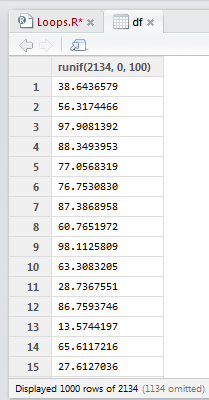
Here's a quick example of what I was dealing with. Take this data frame that has 2134 rows of random numbers between 0 and 100. The start of the data frame is shown.

The code shows a simple for loop that is to iterate through each row and turn each value in an even row to zero. This is achieved using the modulo operation of row number (i) %% 2. If a remainder remains, then the row is odd. No remainder, the row is even.

After running the loop, there is no change to the values in the data frame. WHY?

I don’t know what neuron fired in my head, but it set off a cascade of action potentials that made me want to slap palm against forehead (my palm, my forehead, not someone else's). I had forgotten this.

That's right. A "1" followed by a ":" before nrow(df). Previously I had "i in nrow(df)" assuming that this was sufficient for R to know I wanted it to iterate through each row of the data frame. However, nrow(df) equals the number of rows df, which is 2134. Before, my code read "i in 2134", restricting any changes to the last row alone.

With the correct "i in 1:nrow(df)" the code now reads "i in 1, 2, 3, 4, 5… 2134". The sequential rows of the data frame are specified. 

I felt rather stupid and shared this with a friend. His reply:

Ah yes, I know those moments. And I'm never sure if I should feel smart that I figured it out, or dumb that I made the mistake in the first place :)   

I settled for a bit of both.

Earlier today a new loop was failing. Turns out I had this.

For the love of pizza – I hadn't even included the "nrow" part around the data frame. That one tipped the scales to the dumb-side.

Git add, commit, push – Github

My first experience using GitHub was met with a sea of confusion. "GitHub is a Git repository web-based hosting service, which offers all of the distributed revision control and source code management (SCM) functionality of Git as well as adding its own features" [1]. It's used by my MOOCs for grade assessment. Students upload completed assignment files (such as code text documents and images) to GitHub, made available for viewing by other students. I submitted an assignment for the Reproducible Research course and pleasantly discovered that the GitHib submission went smoothly. This was largely due to recalling I needed to be in the right directory. The following are the steps I took to submit my work to GitHub. I have assumed the reader has set up a GitHub account and has installed Git Bash on their Windows machine [2].

First I was instructed to "fork" a repository. I need to define some terms here. A repository is "a central location in which data is stored and managed" [1]. "A fork is a copy of a repository. Forking a repository allows you to freely experiment with changes without affecting the original project" [3]. I won't go into the details, but to fork a repository, you follow the GitHub link to the repo (that's what the cool kids call it) and click on "Fork". That's it. The forked repo appears in your list of repositories. The contents of the forked repo are available to you to view. But you are not ready to make changes to the contents of these files and make these changes available to others. In order to do that, a local copy of the repo is required on your computer. In other words, the repo and its contents need to sit in a directory on your computer. The local copy and the repo on GitHub are linked. Changes made to the local copy can be synced with GitHib.

To make a local copy of a repo, you need to clone the repo.

Opening Git Bash [4] I typed "git clone" [5], space then a URL. The URL points to the forked repo (called "RepData_PeerAssessment1"). My username on Git is "DataMoose".

After hitting Enter, the repo appears in my Home directory, as seen below with the folder called "RepData_PeerAssessment1".

When I open the folder I can view the contents. Note that there exists a "PA1_temlpate.Rmd" file. Later I will overwrite this file.

I stated that knowing what directory I was in was for smoother sailing. To check the current directory, type "pwd" (which stands for "print working directory").

I'm in my Home directory at C/Users/Karim [6]. I need to change the directory and point to the repo on my machine. Changing directories is achieved by type "cd" followed by a space, then the folder name (that exists in the current directory) I wish to jump into. Hit Enter.

As a sanity check, type "pwd" again to confirm you are now in the desired directory. A very useful thing to type to get a feel for this directory is "git status" [7]. This returned a status on whether any files in the repo had been modified.

Upon completing my assignment, three files ("PA1_template.Rmd", "PA1_template.html", "PA1_template.md") and a folder ("PA1_template_files") contained figures were produced. I copied then pasted the files and folder into my local repo folder, overwriting the "PA1_temlpate.Rmd" file.

Typing "git add ." will add any new or changed files to git. One can add a specific file by typing out the filename. Use of "." Will add all files in the directory.

Typing "git commit –m" will, I suppose, commit the additions. I'm assuming this step is equivalent to asking "Are you sure you wish to continue?". The "first commit" is my choice of statement. I could write anything and it will display on GitHub. After hitting Enter, the files that are added/committed are listed.

Typing "git push –u origin master" then hitting Enter will prompt for your GitHub username and password. After (correctly) keying these in, stuff (hopefully) appears to indicate that the files have been added to the repo on GitHub.

Refreshing your GitHub repo list, you will see that the new/changed files have appeared (those with "first commit").

That's how we fork, clone, add, commit, push with Git. GitHub is a fantastic (free) tool for version control of your work. In the event you made a blunder, you can rollback to prior versions of files. For my purposes, students can hopefully award me full grades for my assignment.

References and notes

1. I Googled this.

2. I haven’t really assumed this. I'm quite aware people use Macs. I'm a PC, and I wear glasses.

3. Help from: https://help.github.com/articles/fork-a-repo/

4. Allow me a moment to get all colloquial on your ass. Git Bash is an interface that lets me type in single line commands that gets the computer to do stuff, OK? OK!

5. As guided by: https://help.github.com/articles/fork-a-repo/

6. My name is Karim. Nice to meet you.

7. I was guided by: http://guides.railsgirls.com/github/

References and notes

Wednesday, 12 November 2014