Probably a better way – Year one

It’s been a year since my first post, and a lot has changed. Looking over my early posts, I’m amused that I started with VBA in Excel. At the time I had completed a VBA training course and was writing a program at work. I saw a future of working exclusively in VBA – writing VB scripts where my customers would use my awfully clunky workbooks to manage and analyse their data. I suspect if I searched “VBA” across job ads, the number of hits has reduced since a year ago.

Soon I commenced the Data Science courses on Coursera. I learnt to program in R via these courses (aided with prior Matlab knowledge) then applied this knowledge at work. I managed my data with R and visualised data with R. I even built a web app (using the Shiny package). R is great, and it’s free. Not like how Facebook is free where one hands over personal data. R is proper free.

I am regularly using R in my new role. I do wonder whether I should learn Python. My understanding is that Python excels over R in web applications and text analytics. I wish I knew Javascript – I would like to create custom interactive displays.

I’d love to know more about statistics and multiple regression. Not entirely sure how I would apply this knowledge. At the heart of it, I’d like to be in a position to receive a large amount of data and simply know what statistical methodology I should be applying towards uncovering insights. I have commenced reading my thick stats book mentioned in this post.

At the moment I am being exposed to different data types and methodologies at work. JSON, XML, MySQL. I’ll take them as they come. I’m fortunate that I am surrounded by developers that have advice when I get stumped. I just have to be more comfortable with asking for help.

Summary: Year one was moving away from VBA to R. Here’s to year two!

Visual display with pivot tables – Excel VBA

The example I use here is terribly simple. Yet a collection of simple techniques can create complexity. Let's colour in data from a pivot table using VBA code. I have the dates of when Breaking Bad episodes aired in the States [1]. I want to see, via a calendar-style display, when these episodes aired over the years of sheer television awesomeness.

Here is the data. The text in blue is text I modified or created. The dates from Wikipedia had to be reformatted to DD/MM/YYYY format. I then used the =Year(), =Month() and =CONCATENATE() formula to get the dates into Year-Month format.

I selected all of the data and created a pivot table (Insert tab, then "PivotTable"). On the right hand "PivotTable Field List" panel, I dragged in "No. in series" under “Column Labels, dragged in "Year-Month" under "Row Labels" and selected the Count of No. in series under "Values". You will see the episode series numbers 1 to 62 across the columns, and the Year-Month down the rows. The "1" in the cells indicate that the respective episode aired on the row's Year-Month.

To get a better representation of time, I included the Year-Months that did not air a Breaking Bad episode by inserting rows. These are shown in blue.

Next, I prettied things up. Added headers for the seasons and Year-Months, and included grid lines. I narrowed the column widths to make square cells. Notice that going down the rows, for each year there are twelve cells (January to December).

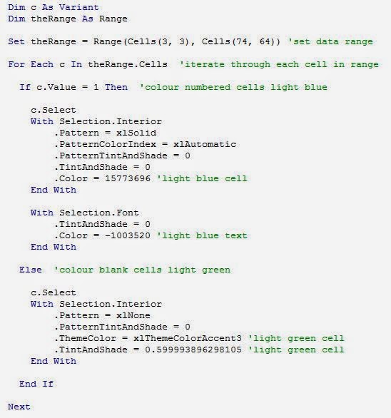
Now for some colour. I want the cells with "1" to be blue, and the blank cells to be green. Since there are few cells with 1, I could simple highlight all cells green then colour the 1 cells blue (and change the "1" text colour to the same blue). That's fine for a one-off, but I intend to repeat the process again, thus I wrote code.

I'll point out some features. Set theRange = Range(Cells(3, 3), Cells(74, 64)) sets the range of cells in the grid that the code will focus on [2]. For Each c In theRange.Cells will point the code to iterate through each cell in the range and do something. That something is colour blue if the cell contains "1", or colour green if the cell in blank. There are three sections that are enclosed with "With" and "End With". The first will turn the cell blue. The second will turn the text colour blue. That last will turn the cell green. After running the code, we get the following.

What is clear from this display is that there simply wasn't enough Breaking Bad episodes. Maybe I'm just sad that there will be no more. I do have the minisodes to watch. And there's Better Call Saul, so yeah!

You may be thinking, what was the point of this display? It's doesn't show that much. This approach may be useful for other purposes. I have used this approach to indicate events over time, such as attendance at a venue or receipt of a service. Provided that the data contains dates, conversion to Year-Month format then use of the pivot table will create the grid structure. The code is to automate the colouring. In my example .Color = 15773696 is light blue cells and .Color = -1003520 is light blue text. .ThemeColor = xlThemeColorAccent3 and .TintAndShade = 0.599993896298105 is for light green colouring. To get the codes for different colours, turn on the "Record Macro" feature (Developer tab), select the desired colour, stop the recorder and take a look at the macro produced for the respective codes for colour to copy and paste into your code.

My pivot table only contains one number. With a variety of numbers, one can apply Conditional Formatting (Home tab) to get various shades of colour. Darker shades indicate higher numbers. One could produce something like this display, yet I don't know what software was used to produce it [3].

Excel is great for simple visual displays, but I am exploring alternatives. I'll start with R and will let you know how it goes.

References and notes

1. Data from Breaking Bad Episodes Wiki page.

2. I hard-coded the cell position numbers for this particular dataset. One can set the code to use relative cell positions.

3. I came across the display via this Reddit thread. It was produced by Project Tycho. The original image was modified by user FortyFs, which I used in this post.

Call a procedure to get the first empty column number – Excel VBA

You have a spreadsheet and you want to add some data in the first empty column. How do you know which column to use? You simply use your eyes and look. Guide your mouse to move the cursor to a cell in the empty column, enter a formula, then autofill down. But how does one automate this for a spreadsheet when you do not know beforehand which column is empty (eg column B, column AB, etc)? Your computer does not have eyes to simply check.

Or does it?

A webcam is an eye, but your webcam will not assist you with automation. It will assist you with a fine evening on Chatroulette.

Below is code to determine the location of the first empty column in a spreadsheet. As a bonus, it includes code that will determine the last row where data exists on the spreadsheet [1].

Take the following sheet which holds episode details of Breaking Bad season 1 [2].

After running the code, it returns the next empty column (emptyCol) as column 5 (column E), and the last row with data as row 8. 

Now I want to populate column 5 (column E) with data. Using the Original air date, I want to list the year. I can use something like this:

Range(Cells(2, emptyCol), Cells(rowLast, emptyCol)).Formula = "=Year(Originalairdate)"

Where emptyCol = 5, rowLast = 8. The “Range(Cells(), Cells())” part are the coordinates of the range where I wish to populate cells: from rows 2 to 8, restricted to column 5. I have used the year formula on the data in the “Original air date” column [3]. 

Next scenario. What happens when you have to repeat this action? I now want to have a column with the month of the original air date (using the Month() formula), and then populate the next empty column with the day (using the Day() formula). This would be populated in column F and G respectively. Before populating data in the next empty column, the software needs to know where the empty column is. Like this:

• Find the column number of the next empty column
• Remember the column number
• Point to empty column using the remembered column number
• Populate with data (eg year)
• Find the column number of the next empty column
• Remember the column number
• Point to empty column using the remembered column number
• Populate with data (eg month)
• Find the column number of the next empty column
• Remember the column number
• Point to empty column using the remembered column number
• Populate with data (eg day).

Each time a column is populated with data, the empty column number changes by one (year in column 5, month in column 6, day in column 7). You could copy and paste the whole code each time to get the next empty column (and last row with data if this changes). Or, you could set the code aside in a procedure. When you need to run the code, call the procedure. Here I have placed the code in a procedure called "EmptyCol_LastRow". 

I can call this procedure (EmptyCol_LastRow) as required to get the new emptyCol values, as follows:

• Call procedure to get emptyCol and lastRow
• emptyCol = 8, lastRow = 8
• Populate with year
• In column 8 
• Call procedure to get emptyCol and lastRow
• emptyCol = 9, lastRow = 8
• Populate with month
• In column 9
• Call procedure to get emptyCol and lastRow
• emptyCol = 10, lastRow = 8
• Populate with day
• In column 10.

The corresponding code that populates the columns with data is shown below.

Rather than copy paste lines of code to get updated column and row numbers, simply call the procedure as required!

References and notes

1. Code modified from ozgrid.com VBA/ExcelRanges page. 

2. Data from Breaking Bad Episodes Wiki page.

3. I manually created a named range for the Original air date column called “Originalairdate”.

Find word matches across two sheets – Excel VBA

We have an Incidents registry where staff members can note down any work, health and safety (WHS)/ occupational health and safety (OHS) events that occur on-site. These can be innocuous (paper cut) to the severe. Here is a simple list of incidents with dates on a worksheet called “Incidents”.

I was asked to provide a subset of this sheet containing any incidents that made mention of "WHS" (red text). I could also highlight any mention of "OHS" (magenta text), though this was secondary. The real list I worked off had many thousands of rows (and no coloured text). What did I do to find the targets "WHS" and "OHS" (including "WH&S" and "OH&S")? I used Ctrl F then marked the cell next to the incident with "1". At the end, I could sort by these numbers and remove rows that contained none – hence subsetting the data as required.

As I Ctrl F'ed and contemplated my life in general, I knew I would have to perform a similar task on a different spreadsheet in the future. Did someone say coding solution?

I built something! After running the code to search for "WHS", "WH&S", "OHS" and "OH&S", I get the below results.

First I created the Target sheet which contains the list of words/terms that I wish to find on the Incidents sheet. Column A lists the primary target words to search for. If either "WHS" or "WH&S" are found, the incident row will be marked with "1".Column B lists the secondary targets. If either "OHS" or "OH&S" are found on the incident row AND the row IS NOT marked with "1", then the row will be marked with "2" (I do not want to overwrite any existing marks).

I shall pause here. For those who wish to see the code [1], I have (poorly) screen-grabbed it at the end of this post [2]. For those still with me – I will attempt to translate the code steps into words. I'll do this is two parts - Part 1: Sections of code, and, Part 2: Details of code.

Part 1: Sections of code

The code is composed of three key sections: 

1. For c = 1 To colLast (red vertical line).

2. For r = 1 To rowLast (blue vertical line).

3. With Worksheets(“Incidents”).UsedRange (green vertical line).

For c = 1 To colLast iterates through each column on the Target sheet.

For r = 1 To rowLast iterates through each row within each column on the Target sheet.

With Worksheets(“Incidents”).UsedRange interrogates the cells that contain data on the Incidents sheet.

The order of what happens is:

1. First column on the Target sheet is selected (column A).

2. First row in the column on the Target sheet is selected (row 1, column A). A target word is selected ("WHS").

3. The target word is used to find all matches on the Incidents sheet (rows 4, 5, 9, 11, 12) and marks these with "1".

4. The next row in the column on the Target sheet is selected (row 2, column A). The next target word is selected (“WH&S”).

5. The target word is used to find all matches on the Incidents sheet (rows 5, 12) and marks these with "1".

6. The next column on the Target sheet is selected (column B). 

7. The next row in the column on the target sheet is selected (row 1, column B). A target word is selected ("OHS").

8. The target word is used to find all matches on the Incidents sheet and marks these with "2". However, if a row already contains a match value, then it will not overwrite this value (only row 7 will be marked with "2").

9. The next row in the column on the Target sheet is selected (row 2, column B). The next target word is selected ("OH&S").

10. The target word is used to find all matches on the Incidents sheet and marks these with "2" if there is no prior marked value (no additional rows will be marked with "2").

And that's it! All of the words on the Target sheet have been grabbed and used to find a match on the Incidents sheet.

Part 2: Details of code (I'm impressed you're still reading)

Remember: the Target sheet contains the words I am trying to find on the Incidents sheet. The below steps follow the lines of code from top to bottom.

• Determine the last column with data on the Target sheet. Why? I need to know how many columns there are to search across for target words – otherwise I would search endlessly and freeze the program. There are 2 columns in the Target sheet, A and B.
• For each column on the Target sheet, determine the last row with data. Starting with column A, the last row with data is row 2.
• Since I now know the column number (1) and the last row with data (2) in the column (column A), I can get the range of the column. I will select my target words from this range to begin. If I used the whole worksheet range, I would inadvertently start selecting blank cells to find target words. Since each row of the Incidents data contains blank spaces, each row would be marked with "1", which I do not want. Setting ranges involve knowing exactly where the data you wish to use is located.
• Activate the Incidents sheet. A user can activate a sheet simply by selecting that sheet. Once the code has activated the sheet, any action by the code will apply to the Incidents sheet (unless specified otherwise).
• Get the first empty column of Incidents sheet. Why? Because this is where the mark values will be populated each time a target word is found. I do not wish to populate the values in a column that contains data.
• Set initial values for variables. I have two – rowLoc and firstRowLoc. Before describing these, I should note the code is driven by a range called Loc (I have underlined in red where this appears in the code below). Loc gets the cell location (range) where the target word match was found. I can get the row number of where Loc exists via rowLoc = Loc.row. firstRowLoc is the row where the first instance of a target word match was found. Before I begin to use rowLoc and firstRowLoc, I have to set initial values (they cannot be blank). rowLoc = 0 and firstRowLoc = -1 and I'll explain why I used these values below.
• Specify the range to use when searching for target words in the Incident sheet. The code will not search outside of this range.
• Select a target word from the target range. Recall above that the range of column A listed words has been determined. The first target word “WHS” is chosen.
• Set Loc to find the row where the target word exists on the Incidents sheet. The first instance of where “WHS” is found is on row 4. At this point, the values of rowLoc and firstRowLoc are updated to both equal "4" (no longer 0 and -1, respectively). 
• Enter the Do Until loop. The Do Until loop will continue until the rowLoc = firstRowLoc. In other words, when the Loc returns to the first row where a target word match was found, the condition of rowLoc = firstRowLoc is met, and the loop ends. Had rowLoc and firstRowLoc both been initialised with 0 at the start, then this condition (rowLoc = firstRowLoc; 0 = 0) would have been met and the Do Until loop would not have commenced. Hence prior to the loop, rowLoc = 0 and firstRowLoc = -1 (unequal values). But wait! The previous step indicated that both rowLoc and firstRowLoc equalled 4. If this rowLoc = firstRowLoc condition is now met, shouldn't the loop end? No, because there is a code further on that will find the new target word match and update the rowLoc value (to "5"). Thus when entering the loop again, rowLoc (5) will not equal firstRowLoc (4) and the loop will continue. 
• Still in the loop, when a match is found, mark with "1" if target words are from column A. Otherwise, mark with the column number for column B onwards. That is, if the word is "OHS" or "OH&S", this arises from column B, which is the second column. Hence, the mark value is "2". BUT – only mark with "2" if there is no prior value of "1".
• Set Loc again to get the location of the cell where the target word is found next. Get the row number of where the next word will be found. This is where the rowLoc value is updated (to "5"). Upon entering the loop again, this next rowLoc value will be compared against the firstRowLoc value. If the values match, that means the FindNext code has pointed back to the row where the first match was found, and the loop will end. This allows the next target word to be selected and the code re-enters the loop to interrogate the Incidents data to find a match.
• The process repeats until all words on the Target sheet have been selected and assessed for a match on the sheet.

I probably should have used more screen-grabs for Part 2. My bad.

The code

References and notes

1. I modified code I found on the stackoverflow thread Find all matches in workbook using Excel VBA by Nanashi.

2. The code in the Excel IDE ran over the page. I screen-grabbed two separate sections, pasted it in Word to recombine, made some annotations, then screen-grabbed the combined image. A copy of a copy made is a poor copy. I assume there is a better way to have produced this.

Using named ranges to modify data – Excel VBA

Do you regularly receive spreadsheets with data that needs your analysis expertise? Upon the sheets' return, do you find yourself trudging through the same processes of using formulas, sorting data, arranging tables and producing charts? I am assuming you use a recorded macro which when played back, will execute the series of steps to process the data. That's all fine, until the spreadsheet format changes (ie new columns are added) or a new type of analysis method is required.

This is why I learnt to write VBA (Visual Basic for Applications) code in Excel to create programs that can accommodate anticipated changes.

My first hurdle when working with VBA was to find a way to select a particular column via the column name, and then modify the data.

Take a look at the data below [1]. It shows the average weekly earnings across five private sectors over May/Nov periods. To manually apply a named range to each column, the column range is highlighted then the desired name is typed into the Name Box (red box). This is a not-so-fine procedure with hundreds of columns.

A saner solution is to use dynamic named ranges. A colleague provided his code (which he modified from code he found online), which I in turn modified for my purposes. After running the code, the column names become named ranges [2].

Check this by clicking the Name Manager button (or Ctrl + F3). Notice that the spaces that existed in the column names are replaced with an underscore, and commas have been removed (there are rules for permitted named ranges).

This particular code will select the whole column for the named range (that's what the "!C" does). I will need to apply changes to data on a single cell rather than the whole column. I'll show you how I can point to a single cell.

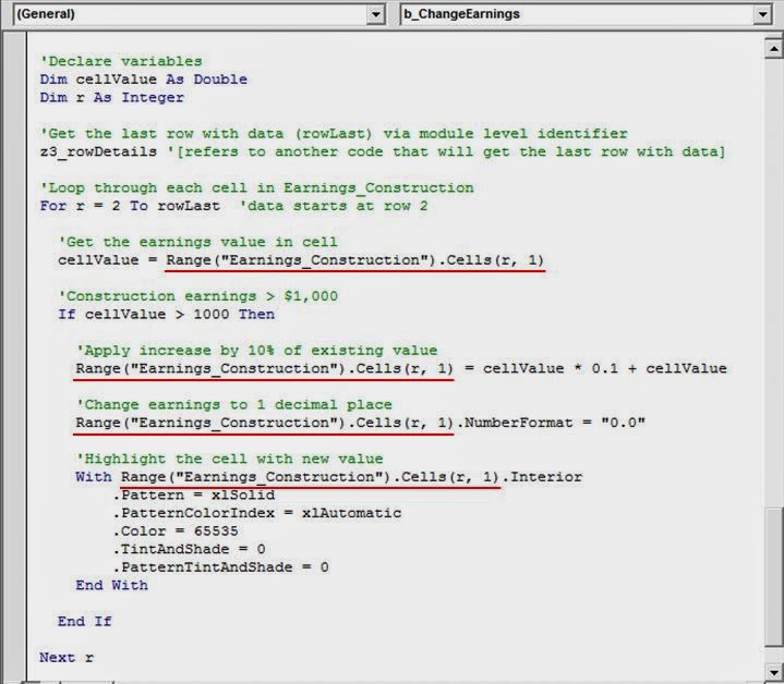
We have named ranges using column titles – Great! Now what? We need a task to perform. Let's say that we have been told that any earnings from the construction sector greater than $1,000 requires updating by 10% of their current value. Below is the code that will loop (one cell at a time) through the Earnings_Construction named range, change the value to one decimal place and highlight the changed cell.

Here's what the results look like after I have run the code.

Look back at the code and focus on the comments (green text) to get a general idea of what each section is doing to the data. If you are unfamiliar with loops, just know that within this loop, for the specific range of cells (the Earnings_Construction named range that holds data), changes are made one cell at a time if the logical conditions are met (earnings are greater than $1,000).

Notice the Range("Earnings_Construction").Cells(r, 1) (red underline). This is where I used the named range to manipulate data. Breaking it down, Range("Earnings_Construction") is the whole named range (the whole column). Since I have a For loop that will use data one cell at a time, the .Cells(r, 1) appended to the named range will point to the single cell. For (r, 1), the r is the current row in the loop, and the 1 is the column number of the range (the named range exists in a single column, hence 1). When r = 3, the value in cell row 3 of the named range (868.9) will be the focus.

The first time Range("Earnings_Construction").Cells(r, 1) is used, the value of the cell is assigned to cellValue. When I call cellValue, the value of the cell is returned. For the remaining three occasions, if the condition of > 1000 is met, the value in the cell will be increased by 10%, have the decimal place set to one, and the cell will be highlighted. 

If someone was to come by and insert a bunch of new columns all over the place, the code will still work. This is because it uses the column name to create the named range independent of new columns. However, the column title must stay the same (ie “Earnings Construction”) each time data is received. If the names changes, send the data back (or be nice and change the column name yourself).

References and notes

1. Data modified from the Australian Bureau of Statistics. TABLE 10G. Average Weekly Earnings, Industry, Australia (Dollars) - Original - Persons, Full Time Adult Ordinary Time Earnings.

2. The screengrab does not show all the details required to run the code. I've displayed it primarily for the comments (green text) to get a general sense of what the code is doing.