Using named ranges to modify data – Excel VBA

Do you regularly receive spreadsheets with data that needs your analysis expertise? Upon the sheets' return, do you find yourself trudging through the same processes of using formulas, sorting data, arranging tables and producing charts? I am assuming you use a recorded macro which when played back, will execute the series of steps to process the data. That's all fine, until the spreadsheet format changes (ie new columns are added) or a new type of analysis method is required.

This is why I learnt to write VBA (Visual Basic for Applications) code in Excel to create programs that can accommodate anticipated changes.

My first hurdle when working with VBA was to find a way to select a particular column via the column name, and then modify the data.

Take a look at the data below [1]. It shows the average weekly earnings across five private sectors over May/Nov periods. To manually apply a named range to each column, the column range is highlighted then the desired name is typed into the Name Box (red box). This is a not-so-fine procedure with hundreds of columns.

A saner solution is to use dynamic named ranges. A colleague provided his code (which he modified from code he found online), which I in turn modified for my purposes. After running the code, the column names become named ranges [2].

Check this by clicking the Name Manager button (or Ctrl + F3). Notice that the spaces that existed in the column names are replaced with an underscore, and commas have been removed (there are rules for permitted named ranges).

This particular code will select the whole column for the named range (that's what the "!C" does). I will need to apply changes to data on a single cell rather than the whole column. I'll show you how I can point to a single cell.

We have named ranges using column titles – Great! Now what? We need a task to perform. Let's say that we have been told that any earnings from the construction sector greater than $1,000 requires updating by 10% of their current value. Below is the code that will loop (one cell at a time) through the Earnings_Construction named range, change the value to one decimal place and highlight the changed cell.

Here's what the results look like after I have run the code.

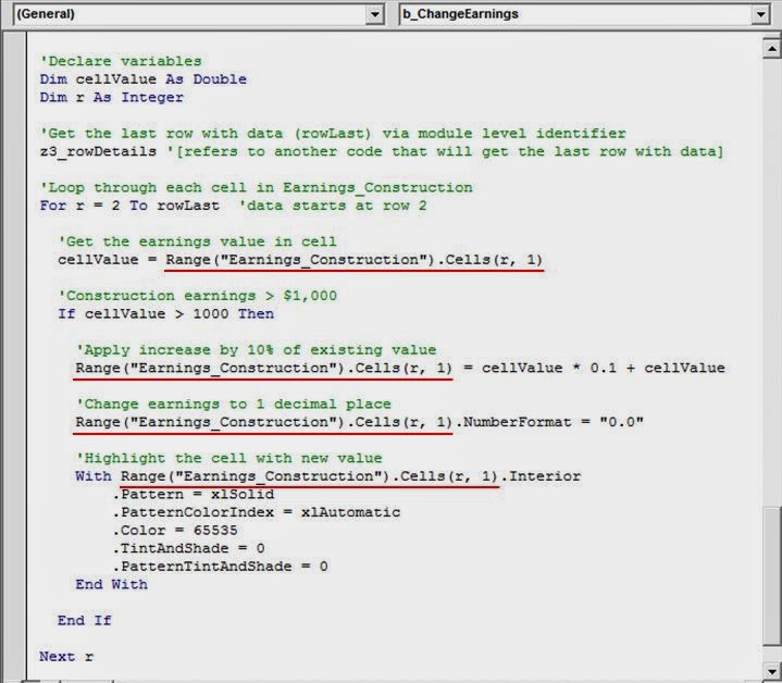
Look back at the code and focus on the comments (green text) to get a general idea of what each section is doing to the data. If you are unfamiliar with loops, just know that within this loop, for the specific range of cells (the Earnings_Construction named range that holds data), changes are made one cell at a time if the logical conditions are met (earnings are greater than $1,000).

Notice the Range("Earnings_Construction").Cells(r, 1) (red underline). This is where I used the named range to manipulate data. Breaking it down, Range("Earnings_Construction") is the whole named range (the whole column). Since I have a For loop that will use data one cell at a time, the .Cells(r, 1) appended to the named range will point to the single cell. For (r, 1), the r is the current row in the loop, and the 1 is the column number of the range (the named range exists in a single column, hence 1). When r = 3, the value in cell row 3 of the named range (868.9) will be the focus.

The first time Range("Earnings_Construction").Cells(r, 1) is used, the value of the cell is assigned to cellValue. When I call cellValue, the value of the cell is returned. For the remaining three occasions, if the condition of > 1000 is met, the value in the cell will be increased by 10%, have the decimal place set to one, and the cell will be highlighted. 

If someone was to come by and insert a bunch of new columns all over the place, the code will still work. This is because it uses the column name to create the named range independent of new columns. However, the column title must stay the same (ie “Earnings Construction”) each time data is received. If the names changes, send the data back (or be nice and change the column name yourself).

References and notes

1. Data modified from the Australian Bureau of Statistics. TABLE 10G. Average Weekly Earnings, Industry, Australia (Dollars) - Original - Persons, Full Time Adult Ordinary Time Earnings.

2. The screengrab does not show all the details required to run the code. I've displayed it primarily for the comments (green text) to get a general sense of what the code is doing.

Probably a better way

I analyse data. When faced with data in spreadsheets, a typical first-step analysis approach is to organise the rows and columns with Excel formulas to produce averages that feed into bar plots. If one has time, a measure of variance (error bars) can be included. An assumption I hold is that most of data analysis is the organisation and management of said data. Ensuring that data is in a particular format will permit an applied algorithm to crunch the numbers in an automated fashion to produce a fancy plot (with error bars).

In this time of "data science" and "big data" (I'm not entirely sure what these terms mean) I am continually questioning if my approach to data analysis is the most efficient (or "correct"). When faced with a programming hurdle, I usually land on answers via Google, write/modify code, then continue until the next hurdle. Whilst I get the job done, I'd love to know if there's better way to work with data.

This blog is a collection of data analysis, management and programming work I conduct across various contexts. I'll refrain from posting lines of code. Instead, I'll describe my approach to solve a particular problem. I suspect that most readers would find my initial solutions haphazard, off-the-mark, inefficient, or possibly cute. That’s OK – I'm hoping readers will provide an alternative method to make life a little bit easier.

In addition, this blog may help me write more awesome-like.